Forest plot of studies with a heatmap of study properties

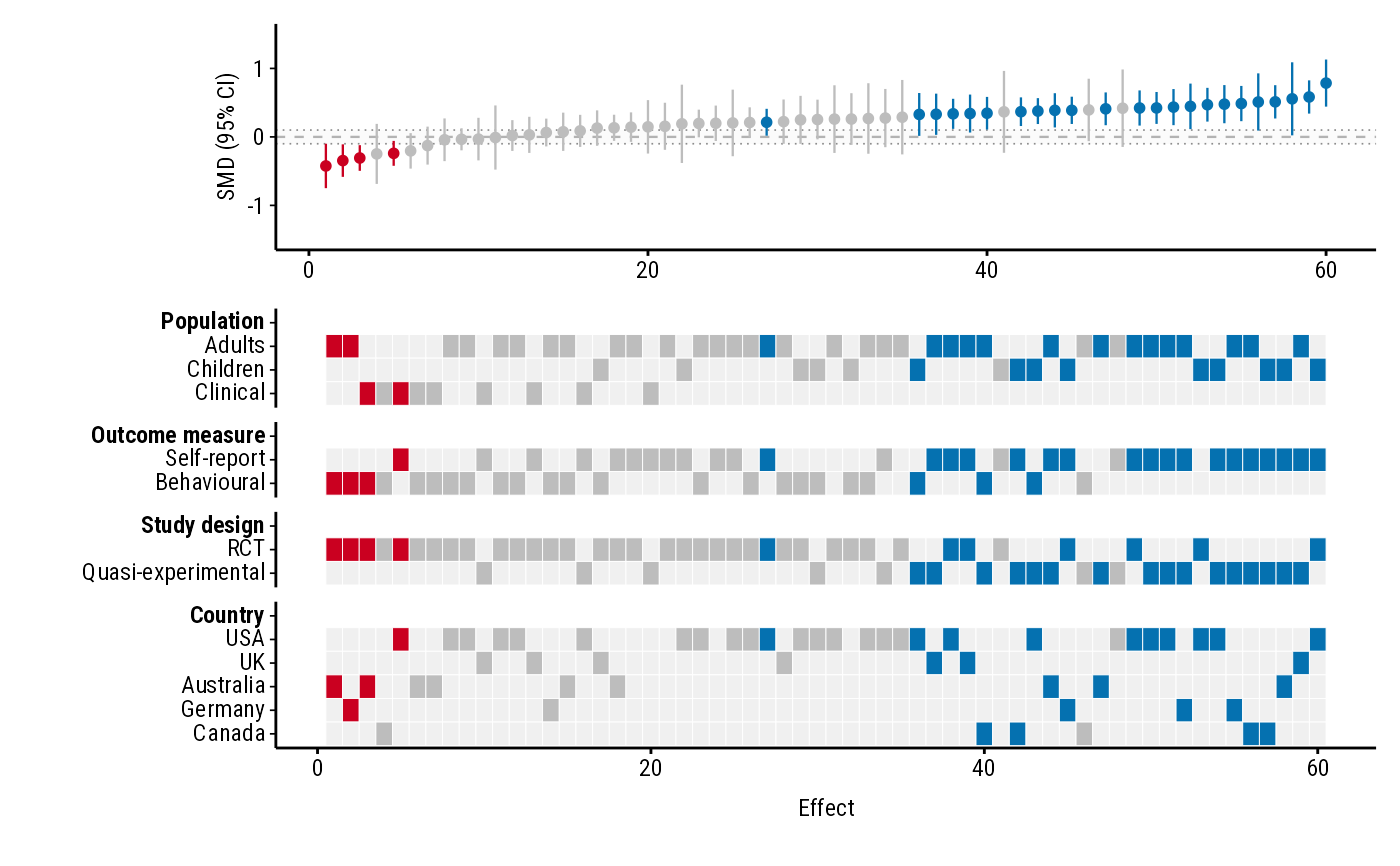
Plots each study's effect size and 95% confidence interval, sorted from smallest to largest, above a heatmap showing each study's properties (population, design, country, ...). It shows at a glance whether studies with particular properties tend to find larger or smaller effects.

Usage

plot_forestmap(
  data,
  es,
  lb = NULL,
  ub = NULL,
  moderators,
  vi = NULL,
  se = NULL,
  font = "Roboto Condensed",
  palette = "default",
  text_size = 9,
  forest_height = "auto",
  null_value = 0,
  rope = NULL,
  y_limits = NULL,
  y_label = "Effect size",
  x_label = "Effect",
  max_levels = NULL,
  layout = c("standard", "compact")
)

Arguments

data: A data frame with one row per study.
es: Name of the column holding each study's effect size.
lb, ub: Names of the columns holding the lower and upper bounds of each study's 95% confidence interval. Give these, or vi, or se.
moderators: Names of the columns holding study properties (factors). Name the vector to set each moderator's heading, e.g. c("Study design" = "design", "Population" = "population"); unnamed entries use the column name.
vi: Name of a column holding each study's sampling variance (e.g. vi from metafor::escalc()). The 95% confidence interval is computed as es ± 1.96 × √vi. Use instead of lb and ub.
se: Name of a column holding each study's standard error. The 95% confidence interval is computed as es ± 1.96 × se. Use instead of lb and ub.
font: A font family installed on your computer (e.g. "Helvetica"), or the path to a .ttf/.otf font file. The default, "Roboto Condensed", comes with the package, so it works on every computer.
palette: A palette name from forestmap_palettes ("default", "okabe_ito", "viridis", "greyscale") or three colours, e.g. c(positive = "darkgreen", negative = "purple", null = "grey").
text_size: Base text size in points.
forest_height: Share of the plot's height given to the forest plot (the top panel), between 0 and 1 (0.5 gives the forest plot and heatmap equal height). "auto" (the default) gives the heatmap more room the more rows it has.
null_value: The value meaning "no effect": 0 for differences and log ratios, 1 for raw ratios such as odds ratios.
rope: Optional region of practical equivalence, drawn as a shaded band: two numbers such as c(-0.1, 0.1), or one number for a band symmetric around null_value.
y_limits: Optional y-axis limits, e.g. c(-1, 1). By default the axis is symmetric around null_value and shows every confidence interval in full; for ratios (null_value above 0 and every value positive) it starts at 0.
y_label, x_label: Axis titles.
max_levels: Optional maximum number of rows per moderator. With max_levels = 3, the 2 most common levels are shown and the rest are merged into one "Other" row. If levels tie for the last place, all of them are kept (with a warning). NULL (the default) shows every level.
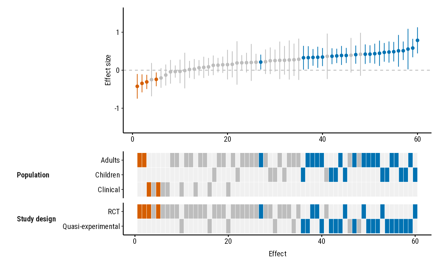
layout: "standard" puts a bold heading above each moderator's rows; "compact" puts the moderator name to the left of its rows instead, which makes the heatmap shorter.

Value

A patchwork object. Print it to display it, or save it with ggplot2::ggsave().

Details

Each row of data is one study. Effects are coloured by their confidence interval: positive when it lies entirely above null_value, negative when entirely below, and null otherwise. Each study's heatmap tiles take the same colour.

Moderators

Each moderator (study property) gets its own block in the heatmap with one row per factor level, in the order of the factor's levels. Use factor() with levels = to control the order. A missing value (NA) means the study doesn't report that property, so it gets no filled tile in that block. Character columns are converted to factors (with a message).

Size and saving

The plot has no fixed physical size; choose the width and height when you save it, e.g. ggplot2::ggsave("plot.png", p, width = 7, height = 5.25). forest_height and text_size control proportions and text.

PNG and SVG files saved with ggplot2::ggsave() always use the chosen font. Some other graphics devices only see fonts installed on your computer, and show the bundled Roboto Condensed in another font until you install it (the files are in system.file("fonts", package = "forestmap")):

RStudio's Plots pane: or set Tools > Global Options > General > Graphics > Backend to AGG.
PDF: save with device = cairo_pdf.

Examples

p <- plot_forestmap(
  forestmap_example,
  es = "smd", vi = "vi",
  moderators = c(
    "Population" = "population",
    "Outcome measure" = "outcome",
    "Study design" = "design",
    "Country" = "country"
  ),
  rope = c(-0.1, 0.1),
  y_label = "SMD (95% CI)"
)
p


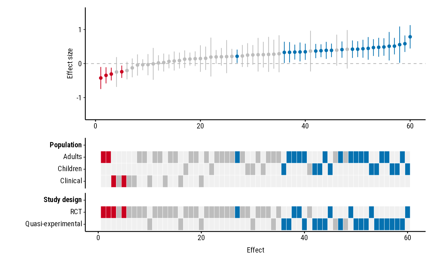
# With confidence interval bounds instead of variances
dat <- forestmap_example
dat$ci_lower <- dat$smd - 1.96 * sqrt(dat$vi)
dat$ci_upper <- dat$smd + 1.96 * sqrt(dat$vi)
plot_forestmap(
  dat, es = "smd", lb = "ci_lower", ub = "ci_upper",
  moderators = c("Population" = "population", "Study design" = "design")
)


# Compact layout, Okabe-Ito palette
plot_forestmap(
  forestmap_example, "smd", vi = "vi",
  moderators = c("Population" = "population", "Study design" = "design"),
  palette = "okabe_ito",
  layout = "compact"
)


if (FALSE) { # \dontrun{
ggplot2::ggsave("forestmap.png", p, width = 7, height = 5.25, dpi = 300)
} # }