Forest Plots with a Heatmap of Study Properties • forestmap

forestmap draws a forest plot with a heatmap of study properties. Each study in your meta-analysis is shown with its effect size and 95% confidence interval, sorted from smallest to largest. Underneath, a heatmap shows each study’s properties (population, design, country, …), so you can see at a glance whether studies with particular properties tend to find larger or smaller effects.

Installation

Install from r-universe:

install.packages(
  "forestmap",
  repos = c("https://shaheedazaad.r-universe.dev", "https://cloud.r-project.org")
)

Example

You need a data frame with one row per study: its effect size, its sampling variance (or standard error, or 95% CI bounds), and one factor column per study property. NA means the study doesn’t report that property.

library(forestmap)
head(forestmap_example)
#>         study   smd      vi   n population     outcome             design
#> 1   Wang 2005 0.470 0.01581 253   Children        <NA>                RCT
#> 2 Hughes 2013 0.261 0.03704 108   Children Behavioural                RCT
#> 3  Rossi 2005 0.510 0.04545  88     Adults Self-report Quasi-experimental
#> 4  Baker 2006 0.410 0.01493 268     Adults        <NA> Quasi-experimental
#> 5 Hughes 2008 0.786 0.03077 130   Children Self-report                RCT
#> 6 Martin 2023 0.260 0.06349  63     Adults        <NA>                RCT
#>     country
#> 1       USA
#> 2      <NA>
#> 3    Canada
#> 4 Australia
#> 5       USA
#> 6       USA

Tell plot_forestmap() which columns are which. Name the properties to set the headings shown in the plot.

plot_forestmap(
  forestmap_example,
  es = "smd",
  vi = "vi",
  moderators = c(
    "Population" = "population",
    "Outcome measure" = "outcome",
    "Study design" = "design",
    "Country" = "country"
  ),
  y_label = "SMD (95% CI)"
)

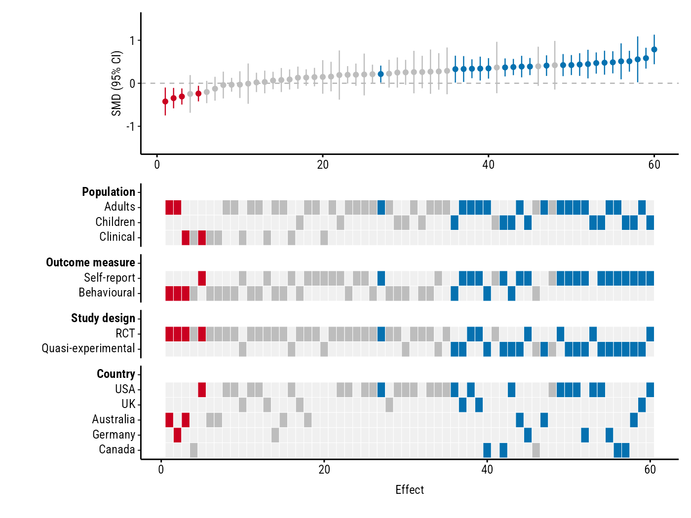
Forest plot of 60 studies sorted by effect size, with a heatmap of population, outcome measure, study design and country below.

Blue studies have a confidence interval entirely above zero, red ones entirely below, and grey ones include zero. In this example, every study with a negative effect is an RCT, while the largest positive effects come mostly from quasi-experimental studies using self-report measures.

You can change the font, colours, text size, layout and more: see Customising the plot. Saving is up to you, e.g.:

p <- plot_forestmap(...)
ggplot2::ggsave("forestmap.png", p, width = 7, height = 5.25, dpi = 300)