Getting started with anovapowersim

anovapowersim simulates power for balanced factorial ANOVA designs. Specify the factors/levels, the term of interest, and a target partial eta squared. anovapowersim generates default term-specific cell means, simulates datasets, refits the ANOVA with stats::aov(), and estimates power.

library(anovapowersim)

Search for the required sample size

The easiest way to get your required sample size is to use power_n() to search for the sample size needed to reach the requested power.

This example is a 2 x 2 mixed design with one between-subjects factor (cond) and one within-subject factor (stim).

We specify that we are interested in the cond:stim interaction, and that we want to have 80% power to detect a partial eta squared of 0.14. power_n() will search for the required sample size per between-subject cell, so n = 13 gives total N = 26.

power_n(
  between = c(cond = 2), # cond has 2 levels
  within = c(stim = 4), # stim has 4 levels
  term = "cond:stim",
  target_pes = 0.14,
  alpha = 0.05,
  power = 0.80,
  n_sims = 1000, # use 5000+ for a more precise estimate
  seed = 123 # for reproducibility
)

#> <anovapowersim_curve>
#>   term:          'cond:stim'
#>   target power:  0.800
#>   alpha:         0.05
#>   effect size:   pes = 0.14
#>   n values:      5 per-cell sample sizes visited
#>   sims per cell size: 1000
#>   SS type:       III
#>   n needed for between-subjects cell: 13
#>   total N needed: 26
#> 
#>  n_per_cell total_n n_sims num_df den_df    ncp power_calc power_sim
#>          10      20   1000      3     54  8.791      0.665     0.665
#>          12      24   1000      3     66 10.744      0.767     0.783
#>          13      26   1000      3     72 11.721      0.808     0.808
#>          15      30   1000      3     84 13.674      0.872     0.882
#>          20      40   1000      3    114 18.558      0.958     0.951

Note: here we use 1000 simulations for a quick example, but the package defaults to 10000 simulations for more precise estimates.

The output table uses compact column names: n_per_cell is the sample size per between-subject cell, total_n is the full sample size, num_df and den_df are the ANOVA degrees of freedom, ncp is the noncentrality parameter, power_calc is the noncentral F power calculation, and power_sim is the simulation estimate.

Adding factors and levels

You can add factors and levels as needed, and specify any term of interest. For, example if we want to add a between condition with 3 levels, and we are interested in the 3-way interaction, we can do:

power_n(
  between = c(cond = 2, age = 3), # cond has 2 levels, age has 3 levels
  within = c(stim = 4), # stim has 4 levels
  term = "cond:stim:age",
  target_pes = 0.14,
  alpha = 0.05,
  power = 0.80,
  n_sims = 1000, # use 5000+ for a more precise estimate
  seed = 123 # for reproducibility
)

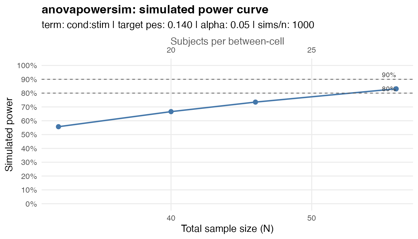
Simulate a power curve

You might want to see how power changes across a range of sample sizes. power_curve() simulates power across a range of sample sizes, which you can specify with n_range. The result is a tidy data frame that you can plot with plot_power_curve().

pc <- power_curve(
  between = c(cond = 2),
  within = c(stim = 2),
  term = "cond:stim",
  target_pes = 0.14,
  n_range = c(16, 20, 23, 28), # n per between-subject cell
  n_sims = 1000,
  seed = 123
)
pc

#> <anovapowersim_curve>
#>   term:          'cond:stim'
#>   target power:  <not specified>
#>   alpha:         0.05
#>   effect size:   pes = 0.14
#>   n values:      4 per-cell sample sizes visited
#>   sims per cell size: 1000
#>   SS type:       III
#>   n needed for between-subjects cell: <not reached>
#>   total N needed: <not reached>
#> 
#>  n_per_cell total_n n_sims num_df den_df   ncp power_calc power_sim
#>          16      32   1000      1     30 4.884      0.571     0.557
#>          20      40   1000      1     38 6.186      0.679     0.666
#>          23      46   1000      1     44 7.163      0.745     0.735
#>          28      56   1000      1     54 8.791      0.829     0.831

Advanced options

Run simulations in parallel

For larger simulation runs, set parallel = TRUE. If you do not set cores, anovapowersim uses one fewer than the number of available cores and prints a message with the chosen count. Set cores explicitly when you want a fixed number of cores.

power_curve(
  between = c(cond = 2),
  within = c(stim = 2),
  term = "cond:stim",
  target_pes = 0.14,
  n_range = c(16, 20, 23, 28),
  n_sims = 5000,
  parallel = TRUE,
  cores = 4,
  seed = 123
)

Match the G*Power convention

By default, anovapowersim calibrates the simulated cell means so the empirical reference dataset has the requested partial eta squared under the fitted stats::aov() model. This corresponds to the fitted ANOVA denominator-df noncentrality convention.

Set gpower = TRUE when you want the G*Power-style convention (when using the ’as in Cohen (1988) option for within-subjects designs) lambda = total_n * f^2.

power_n(
  between = c(cond = 2),
  within = c(stim = 4),
  term = "cond:stim",
  target_pes = 0.14,
  alpha = 0.05,
  power = 0.80,
  n_sims = 1000,
  seed = 123,
  gpower = TRUE
)

#> <anovapowersim_curve>
#>   term:          'cond:stim'
#>   target power:  0.800
#>   alpha:         0.05
#>   effect size:   pes = 0.14
#>   n values:      7 per-cell sample sizes visited
#>   sims per cell size: 1000
#>   G*Power convention: TRUE
#>   SS type:       III
#>   n needed for between-subjects cell: 35
#>   total N needed: 70
#> 
#>  n_per_cell total_n n_sims num_df den_df    ncp power_calc power_sim
#>          28      56   1000      3    162  9.116      0.706     0.695
#>          31      62   1000      3    180 10.093      0.755     0.734
#>          33      66   1000      3    192 10.744      0.784     0.780
#>          34      68   1000      3    198 11.070      0.798     0.796
#>          35      70   1000      3    204 11.395      0.811     0.821
#>          42      84   1000      3    246 13.674      0.883     0.876
#>          56     112   1000      3    330 18.233      0.959     0.967